| MCMD2 |
| MCMD2 |
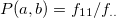
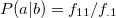
Find out the degree of similarity between two variable fields (distance) at f= parameter, specify the degree of similarity (distance) function at c= parameter to derive the similarity matrix.
msim c= f= [a=] [k=] [-d] [i=] [o=] [bufcount=] [-nfn] [-nfno] [-x] [-q] [precision=] [--help] [--version]
k= Field(s) (multiple items can be specified) specified here is used as the unit of calculation. f= Field names for the calculation of degree of similarities between two fields. c= Specify the similarity measure(s) (distance) (multiple fields can be specified). As shown in the example below, the field name of the similarity measure results can be defined by using a : (colon). If the name of field is not defined with colon, the type of degree of similarity (distance) is used as the field name. Example: msim f=x,y,z c=pearson:Pearson product-moment correlation coefficient, euclid:Euclidean distance,cosine:Cosine Similarity measure=covar|ucovar|pearson|spearman|kendall|euclid|cosine| cityblock|hamming|chi|phi|jaccard|supportr|lift|confMax| confMin|yuleQ|yuleY|kappa|oddsRatio|convMax|convMin a= Specify the field name that indicates the name of the two variables. Specify the two arguments with a comma. Field names fld1,fld2 are used if a= is not defined. -d Output as diagonal matrix and upper triangular matrix. Only the lower triangular matrix of similarity matrix is shown if -d option is not specified, but both upper triangular matrix and diagonal matrix are shown by when -d option is specified.
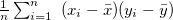
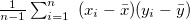
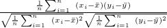
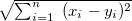
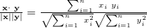
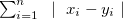
Definition of size for the degree of similarity (or distance) in relation to two real number vectors  is shown in Table 3.25.
Parameter value Detail Distance/similarity Equation definition Range covar Covariance Degree of similarity ucovar Unbiased covariance Degree of similarity pearson Pearson’s product-moment correlation coeff Degree of similarity spearman Spearman’s rank correlation coefficient Degree of similarity kendall Kendall’s rank correlation coefficient Degree of similarity euclid Euclidean distance (number) Distance cosine Cosine Degree of similarity cityblock City block distance Distance hamming Hamming distance Distance
 〜
〜 
 〜
〜
 〜
〜 
 Product-moment correlation coefficient is converted into a ranking 〜
 〜
〜
 〜
〜
 〜
〜
 〜
〜
 〜
〜 
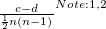
Note 1: 
Note 2: 
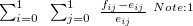
Take the value as 0 or 1, the definition of degree of similarity of two 0-1 vectors  is shown in Table 3.27. The
  symbols used in the table, the value of
  is enumerated in different combinations of (0,1), and shown in Table 3.26.
 contingency table
 |
|
Total |
|
|
|
|
|
|
|
|
|
Total |
|
|
|
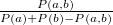
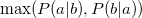
Further, meaning of  is shown below.
|
|
|
|
|
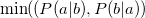
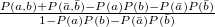
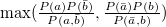
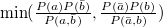
Parameter values Content Distance/similarity Equation Range chi Chi-square value Degree of similarity phi Phi coefficient Degree of similarity jaccard Jack card factor Degree of similarity support Support Degree of similarity lift Value of lift Degree of similarity confMax Maximum confidence Degree of similarity confMin Minimum confidence Degree of similarity yuleQ Ren correlation coefficient of yule (Q) Degree of similarity yuleY Ren correlation coefficient of yule (Y) Degree of similarity kappa kappa Degree of similarity oddsRatio oddsRatio Degree of similarity convMax Maximum conviction Degree of similarity convMin Minimum conviction Degree of similarity
 〜
〜
 〜
〜
 〜
〜
 〜
〜
 〜
〜
 〜
〜
 〜
〜
 〜
〜
 〜
〜
 〜
〜
 〜
〜
 〜
〜
 〜
〜
Note 1:  Note 2:
Calculate the cosine and Pearson’s product-moment correlation coefficient for the combination of two items among x, y, z fields.
$ more dat1.csv
x,y,z
14,0.17,-14
11,0.2,-1
32,0.15,-2
13,0.33,-2
$ msim c=pearson,cosine f=x,y,z i=dat1.csv o=rsl1.csv
#END# kgsim c=pearson,cosine f=x,y,z i=dat1.csv o=rsl1.csv
$ more rsl1.csv
fld1,fld2,pearson,cosine
x,y,-0.5088704666,0.7860308044
x,z,0.1963041929,-0.5338153343
y,z,0.3311001423,-0.5524409416
Calculate the cosine and Pearson’s product-moment correlation coefficient for the combination of two items between x, y, z fields (with d option).
$ msim c=pearson,cosine f=x,y,z -d i=dat1.csv o=rsl2.csv
#END# kgsim -d c=pearson,cosine f=x,y,z i=dat1.csv o=rsl2.csv
$ more rsl2.csv
fld1,fld2,pearson,cosine
x,x,1,1
x,y,-0.5088704666,0.7860308044
x,z,0.1963041929,-0.5338153343
y,x,-0.5088704666,0.7860308044
y,y,1,1
y,z,0.3311001423,-0.5524409416
z,x,0.1963041929,-0.5338153343
z,y,0.3311001423,-0.5524409416
z,z,1,1
Calculate using key field as unit.
$ more dat2.csv
key,x,y,z
A,14,0.17,-14
A,11,0.2,-1
A,32,0.15,-2
B,13,0.33,-2
B,10,0.8,-5
B,15,0.45,-9
$ msim k=key c=pearson,cosine f=x,y,z i=dat2.csv o=rsl3.csv
#END# kgsim c=pearson,cosine f=x,y,z i=dat2.csv k=key o=rsl3.csv
$ more rsl3.csv
key%0,fld1,fld2,pearson,cosine
A,x,y,-0.8746392857,0.8472573627
A,x,z,0.3164384831,-0.521983618
A,y,z,0.1830936883,-0.6719258683
B,x,y,-0.7919009884,0.8782575583
B,x,z,-0.471446429,-0.9051543403
B,y,z,-0.1651896746,-0.8514129252
Using the data with 01 values, compute the phi coefficient and Hamming distance.
$ more dat3.csv
x,y,z
1,1,0
1,0,1
1,0,1
0,1,1
$ msim c=hamming,phi f=x,y,z i=dat3.csv o=rsl4.csv
#END# kgsim c=hamming,phi f=x,y,z i=dat3.csv o=rsl4.csv
$ more rsl4.csv
fld1,fld2,hamming,phi
x,y,0.75,-0.5773502692
x,z,0.5,-0.3333333333
y,z,0.75,-0.5773502692
Using the data with 01 values, compute the phi coefficient and Hamming distance and change the output field name.
$ msim c=hamming:HammingDist,phi:PhiCoeff a=variable1,variable2 f=x,y,z i=dat3.csv o=rsl5.csv
#END# kgsim a=variable1,variable2 c=hamming:HammingDist,phi:PhiCoeff f=x,y,z i=dat3.csv o=rsl5.csv
$ more rsl5.csv
variable1,variable2,HammingDist,PhiCoeff
x,y,0.75,-0.5773502692
x,z,0.5,-0.3333333333
y,z,0.75,-0.5773502692
mstats : Calculate the statistics of one variable.
mmvsim : Calculate sliding window similarity measure.
| MCMD2 |